Forward Propagation
Now we get familiar with the deep feedforward networks’s structure, we are going to learn how the single pass through the network.
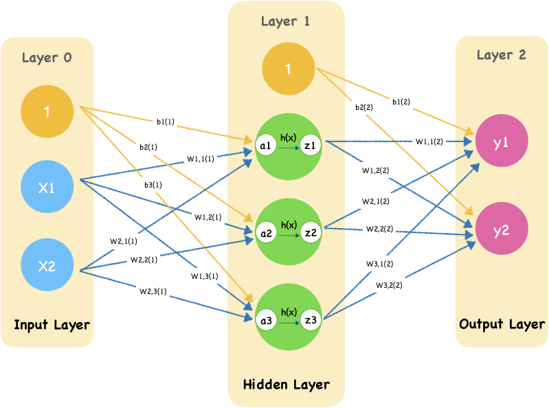
There is a two-layer neural network with one hidden layer. Here the value of input $x_1$ and $x_2$ are:
x1 = 0.2
x2 = 0.8
We start with some random weights and bias from between layer0 and layer1:
# Layer 0 to Layer 1
b1 = 0.4
b2 = 0.56
b3 = 0.64

w11 =1.0
w12 = 0.7
w13 = 0.34
w21 = 0.5
w22 = 0.8
w23 = 0.6

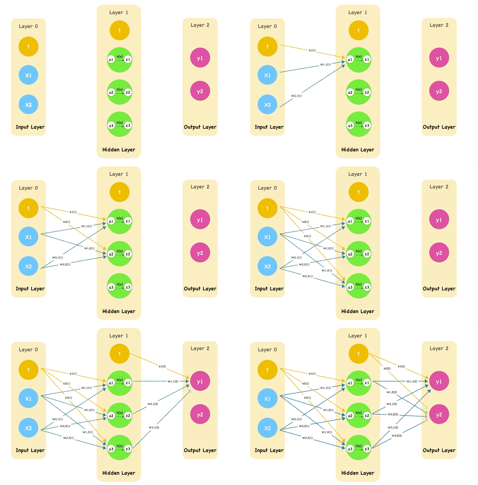
This animation shows how the single pass through the network:

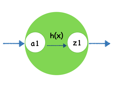
A hidden unit in hidden layer looks like this:

Here we use sigmod function as activate function h(x).
import numpy as np
def sigmoid(x):
    return 1 / (1 + np.exp(-x))
The first layer of nodes is input layer which doing nothing but input signals. Notice that we add a bias node which weight is $b_1$.
Move to the second layer, let’s calculate input of first node:
\[a_1 = w_{1,1}x_1+w_{2,1}x_2 + b_1\]The input nodes have values of 0.2 and 0.8. The weight of bias node in input layer and the first node in hidden layer is 0.4. The weight from second node in input layer is 0.1. The link weight from third node is 0.5. So the combined $a_1$ input is:
\[a_1 = 1 * 0.2 + 0.5 * 0.8 + 0.4\] \[a_1 = 0.2 + 0.4 + 0.4\] \[a_1 =1\]a1 = w11 * x1 + w21 * x2 + b1
print(a1)
1.0
Then we calculate the output of this node using activate function $h(x) = sigmod(x)$.
\[z_1 = sigmod(a_1)\] \[z_1 = \frac{\mathrm{1} }{\mathrm{1} + e^{-1.1} }\] \[z_1 = 0.7310585786300049\]z1 = sigmoid(a1)
print(z1)
0.7310585786300049
Cool! We have finished calculate the first node’s output.
The remaining two nodes can be calculated with the same way.
The second node of hidden layer:
\[a_2 = w_{1,2}x_1+w_{2,2}x_2 + b_2\] \[a_2 = 0.7 * 0.2 + 0.8* 0.8 + 0.4 = 1.3400000000000003\] \[z_2 = sigmod(a_2) = 0.7924899414403644\]a2 = w12 * x1 + w22 * x2 + b2
print(a2)
1.3400000000000003
z2 = sigmoid(a2)
print(z2)
0.7924899414403644
The third node of hidden layer:
\[a_3 = w_{1,3}x_1+w_{2,3}x_2 + b_3\] \[a_3 = 0.34 * 0.2 + 0.6 * 0.8 + 0.4 = 1.1880000000000002\] \[z_3 = sigmod(a_3) = 0.7663831750110293\]a3 = w13 * x1 + w23 * x2 + b3
print(a3)
1.1880000000000002
z3 = sigmoid(a3)
print(z3)
0.7663831750110293
For each node we need to write the corresponding calculation formula, now we just handwritten three nodes, you are likely to get the wrong index. In the future, our network will become more and more complex, and there may be hundreds or thousands of nodes. If we still use such a way, it would be difficult to ensure that nothing goes wrong, isn’t it?
So how do we simplify this? Actually using the matrix in mathematics can simplify and speed up the node’s calculation of the computer. Let’s see what’s going on in next section.